IT Solutions Technology Blog

Rund acht Milliarden Euro weniger sollen dem @bmg_bund für seine Arbeit im kommenden Jahr zur Verfügung stehen. Eine Entwicklung, die bei vielen Beteiligten auf Kritik stößt. Wo gekürzt wird und wo nicht. https://t.co/Wq0GdSTESJ

— kma Online (@kma_online) September 8, 2023

Kalman filter – is a mathematical algorithm used for various purposes such as state estimation and sensor fusion. In Power BI you can use DAX (Data Analysis Expressions) to perform calculations but creating a full Kalman filter implementation would be complex and beyond the scope of a simple example. However you  can provide you with a simplified example of how you might use Power BI to visualize data that has been pre-processed with a Kalman filter

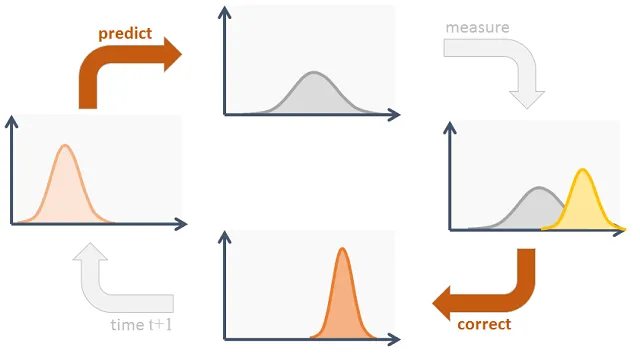
Let’s assume you have a dataset with noisy sensor readings and you want to apply a Kalman filter to smooth out the data before visualizing it in Power BI

Here’s a step-by-step example

Step 1: Data Preparation

Assume you have a dataset in Excel with two columns: „Timestamp“ and „NoisyData“

Step 2: Kalman Filtering

You’ll need to use a programming language like Python or a specialized tool for Kalman filtering to process your data and apply the Kalman filter. Here’s a simplified Python example using the pykalman library

import numpy as np
from pykalman import KalmanFilter

# Load your dataset (e.g., using Pandas)
# Apply Kalman filter to your noisy data
kf = KalmanFilter(initial_state_mean=0, n_dim_obs=1)
filtered_state_means, _ = kf.filter(your_noisy_data)

# Save the filtered data back to a file or database

Step 3: Import Filtered Data into Power BI

After applying the Kalman filter save the filtered data to a new Excel file then import this filtered data into Power BI as a data source

Step 4: Create Power BI Report

Open Power BI and create a new report
Connect to your filtered data source
Create visualizations such as line charts to visualize the filtered data
Here’s a simplified example of what your Power BI report might look like:

Create a line chart with „Timestamp“ on the x-axis and „FilteredData“ (the output of your Kalman filter) on the y-axis

Step 5: Publish and Share

Once you’ve created your Power BI report you can publish it to the Power BI service and share it with others

This example demonstrates how to integrate a Kalman filter into a data preprocessing pipeline and visualize the filtered data in Power BI the actual Kalman filter implementation will require a programming language like Python or a specialized tool

This example assumes a simple 1D position estimation problem

import numpy as np
import matplotlib.pyplot as plt

# Define the true state dynamics (for simulation purposes)
dt = 1.0 # Time step
A = np.array([[1, dt], [0, 1]]) # State transition matrix
B = np.array([[0.5 * dt**2], [dt]]) # Control input matrix
H = np.array([[1, 0]]) # Measurement matrix

# True initial state
x_true = np.array([[0], [0]])

# True state noise covariance (for simulation purposes)
Q = np.array([[0.01, 0.02], [0.02, 0.1]])

# Measurement noise covariance (for simulation purposes)
R = np.array([[1]])

# Number of time steps
num_steps = 100

# Generate noisy measurements
true_states = []
measurements = []

for _ in range(num_steps):
# Simulate the true state dynamics
x_true = np.dot(A, x_true) + np.dot(B, np.array([[np.random.normal(0, Q[0, 0])]]))

# Simulate noisy measurements
z = np.dot(H, x_true) + np.array([[np.random.normal(0, R[0, 0])]])

true_states.append(x_true[0, 0])
measurements.append(z[0, 0])

# Kalman Filter Initialization
x_hat = np.array([[0], [0]]) # Initial state estimate
P = np.array([[1, 0], [0, 1]]) # Initial state estimate covariance

# Kalman Filter Estimation Loop
state_estimates = []

for z in measurements:
# Prediction Step
x_hat = np.dot(A, x_hat)
P = np.dot(np.dot(A, P), A.T) + Q

# Measurement Update Step
K = np.dot(np.dot(P, H.T), np.linalg.inv(np.dot(np.dot(H, P), H.T) + R))
x_hat = x_hat + np.dot(K, z – np.dot(H, x_hat))
P = P – np.dot(np.dot(K, H), P)

state_estimates.append(x_hat[0, 0])

# Plotting
plt.figure(figsize=(12, 6))
plt.plot(true_states, label=’True States‘, linestyle=‘–‚)
plt.plot(measurements, label=’Measurements‘, marker=’o‘, linestyle=’None‘, markersize=5)
plt.plot(state_estimates, label=’Estimated States‘)
plt.xlabel(‚Time Steps‘)
plt.ylabel(‚Position‘)
plt.legend()
plt.title(‚Kalman Filter 1D Position Estimation‘)
plt.grid(True)
plt.show()

Für defekte #Beatmungsgeräte wird der Hersteller @Philips_aktuell ordentlich zur Kasse gebeten. Rund 447 Millionen Euro sprach ein #US-Gericht jetzt allein Klägern mit wirtschaftlichem Schaden zu. https://t.co/JuD5G7ox2l

— kma Online (@kma_online) September 8, 2023

Der Zusatzbeitrag wird wahrscheinlich für einen Durchschnittsbürger um etwa 3 Euro pro Monat steigen. Dafür bekommen wir bessere Medikamente, modernere Technologie, mehr Spezialisierung im Krankenhaus, mehr Digitalisierung. Das muss es uns wert sein. https://t.co/snbhSa1pec

— Prof. Karl Lauterbach (@Karl_Lauterbach) September 7, 2023

Nach der Rotkreuzklinik Lindenberg hat es nun auch die Rotkreuzkliniken München und Wertheim erwischt. Wie die Schwesternschaft München mitteilte, haben die Gesellschaften bereits Anträge auf Einleitung von Schutzschirmverfahren gestellt. https://t.co/064fHlrr94

— kma Online (@kma_online) September 7, 2023